Scaling
Overview
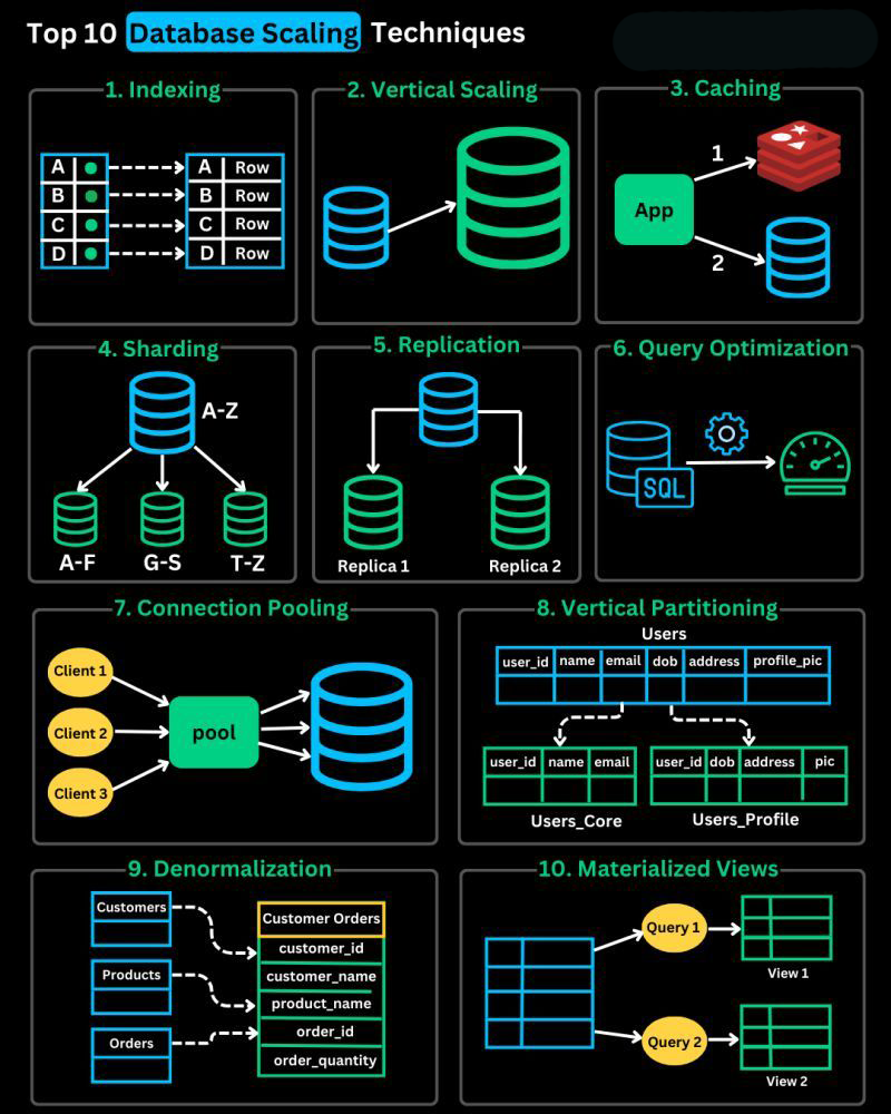
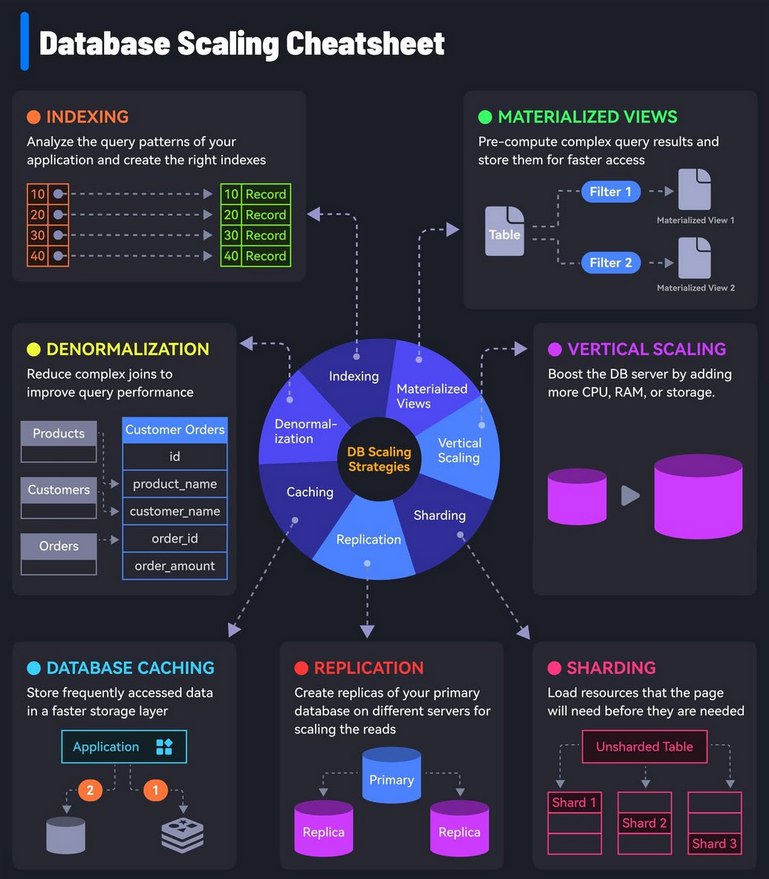
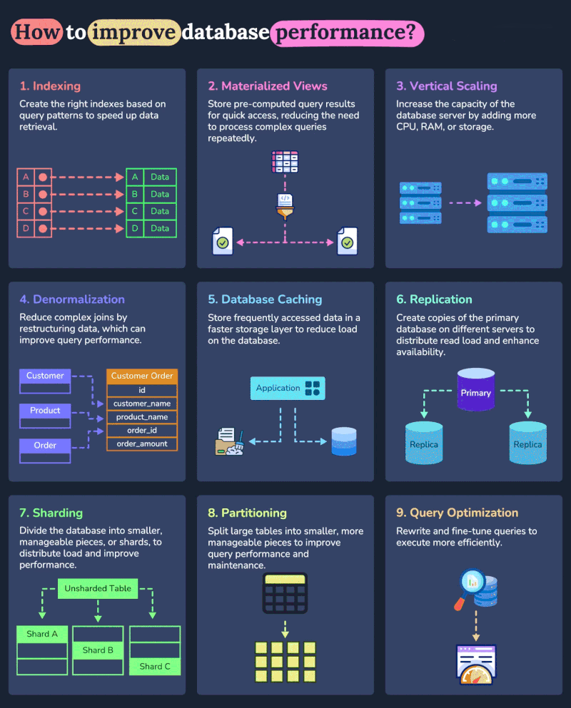
Expand to show Database Scaling Cheatsheet

Sequences
1. Query Optimization (First Priority)
-- Before optimization
SELECT * FROM users WHERE age > 25;

-- After optimization
SELECT id, name FROM users
WHERE age > 25
LIMIT 100;
2. Database Indexing
-- Add indexes for frequently queried columns
CREATE INDEX idx_user_age ON users(age);
CREATE INDEX idx_user_email ON users(email);

-- Composite index for multiple columns
CREATE INDEX idx_user_age_city ON users(age, city);
3. Caching Implementation
# Example using Redis cache
def get_user(user_id):
    # Try cache first
    cached_user = redis_cache.get(f"user:{user_id}")
    if cached_user:
        return cached_user

    # If not in cache, get from DB and cache it
    user = database.query(f"SELECT * FROM users WHERE id = {user_id}")
    redis_cache.set(f"user:{user_id}", user, expire=3600)
    return user
4. Vertical Scaling (Scale Up)
- Increase CPU
- Add more RAM
- Upgrade to faster storage (SSD/NVMe)
5. Database Partitioning
-- Example of date-based partitioning
CREATE TABLE orders (
    order_id INT,
    order_date DATE,
    amount DECIMAL
) PARTITION BY RANGE (YEAR(order_date)) (
    PARTITION p2022 VALUES LESS THAN (2023),
    PARTITION p2023 VALUES LESS THAN (2024),
    PARTITION p2024 VALUES LESS THAN (2025)
);
6. Read Replicas
7. Horizontal Scaling (Sharding)
8. Database Type Optimization
Right choice DB based on demand
Transactions → PostgreSQL/MySQL
Analytics → ClickHouse/Redshift
Caching → Redis
Document Storage → MongoDB
Graph Data → Neo4j
9. Microservices Split
10. Geographic Distribution
US Region:
- Primary DB
- Read Replicas

EU Region:
- Primary DB
- Read Replicas

Asia Region:
- Primary DB
- Read Replicas
Partitioning
1.Types of Partitioning
A. Range Partitioning
-- Partition by date range
CREATE TABLE sales (
    id INT,
    sale_date DATE,
    amount DECIMAL
) PARTITION BY RANGE (YEAR(sale_date)) (
    PARTITION p_2022 VALUES LESS THAN (2023),
    PARTITION p_2023 VALUES LESS THAN (2024),
    PARTITION p_2024 VALUES LESS THAN (2025),
    PARTITION p_future VALUES LESS THAN MAXVALUE
);

-- Partition by amount range
CREATE TABLE orders (
    order_id INT,
    amount DECIMAL
) PARTITION BY RANGE (amount) (
    PARTITION p_small VALUES LESS THAN (100),
    PARTITION p_medium VALUES LESS THAN (1000),
    PARTITION p_large VALUES LESS THAN (10000),
    PARTITION p_huge VALUES LESS THAN MAXVALUE
);
ASCII Visualize
ALL SALES DATA
┌───────────────────┐
│     Database      │
└─────────┬─────────┘
          │
    ┌─────┴─────┬────────────┬────────────┐
    │           │            │            │
┌───▼───┐   ┌───▼───┐   ┌───▼───┐   ┌───▼───┐
│ 2022  │   │ 2023  │   │ 2024  │   │Future │
│ Sales │   │ Sales │   │ Sales │   │ Sales │
└───────┘   └───────┘   └───────┘   └───────┘
B. List Partitioning
-- Partition by region
CREATE TABLE customers (
    id INT,
    name VARCHAR(100),
    country VARCHAR(50)
) PARTITION BY LIST (country) (
    PARTITION p_europe VALUES IN ('France', 'Germany', 'Spain'),
    PARTITION p_asia VALUES IN ('China', 'Japan', 'India'),
    PARTITION p_americas VALUES IN ('USA', 'Canada', 'Brazil')
);
ASCII Visualize
CUSTOMER DATA
     ┌──────────────────┐
     │    Database      │
     └────────┬─────────┘
              │
    ┌─────────┼─────────┐
    │         │         │
┌───▼───┐ ┌───▼───┐ ┌───▼───┐
│EUROPE │ │ ASIA  │ │ USA   │
│France │ │ China │ │ Texas │
│Spain  │ │ Japan │ │ NYC   │
│Italy  │ │ India │ │ LA    │
└───────┘ └───────┘ └───────┘
C. Hash Partitioning
-- Automatically distribute data across 4 partitions
CREATE TABLE users (
    id INT,
    email VARCHAR(100)
) PARTITION BY HASH(id) PARTITIONS 4;
ASCII Visualize
USER DATA (Hash by ID)
┌─────────────────────────┐
│       Database          │
└────────────┬────────────┘
             │
     ┌───────┴──────┐
     │  Hash(ID)    │
     └───────┬──────┘
   ┌─────────┼─────────┐
   │         │         │
┌──▼───┐  ┌──▼───┐  ┌──▼───┐
│ P0   │  │ P1   │  │ P2   │
│ID%3=0│  │ID%3=1│  │ID%3=2│
└──────┘  └──────┘  └──────┘
2. Composite Partitioning (Combining Multiple Types)
-- Partition by year and then by month
CREATE TABLE transactions (
    id INT,
    trans_date DATE,
    amount DECIMAL
) PARTITION BY RANGE (YEAR(trans_date))
  SUBPARTITION BY HASH(MONTH(trans_date))
  SUBPARTITIONS 12 (
    PARTITION p_2023 VALUES LESS THAN (2024),
    PARTITION p_2024 VALUES LESS THAN (2025)
);
ASCII Visualize
SALES DATABASE
        ┌──────────────────────────┐
        │         2023             │
        └───────────┬──────────────┘
                    │
    ┌───────────────┼───────────────┐
    │               │               │
┌───▼───┐       ┌───▼───┐       ┌───▼───┐
│ Q1    │       │ Q2    │       │ Q3    │
└──┬────┘       └──┬────┘       └──┬────┘
   │               │               │
   ├─Jan           ├─Apr           ├─Jul
   ├─Feb           ├─May           ├─Aug
   └─Mar           └─Jun           └─Sep
3. Partition Management
A. Adding New Partitions
-- Add new partition for next year
ALTER TABLE sales ADD PARTITION (
    PARTITION p_2025 VALUES LESS THAN (2026)
);
B. Removing Partitions
C. Reorganizing Partitions
4. Querying Partitioned Tables
A. Partition Pruning (Automatic)
-- Database will only scan relevant partitions
SELECT * FROM sales
WHERE sale_date BETWEEN '2023-01-01' AND '2023-12-31';
B. Partition Selection
5. Best Practices
A. Sizing Guidelines
-- Keep partitions similarly sized
CREATE TABLE logs (
    id INT,
    log_date DATE,
    message TEXT
) PARTITION BY RANGE (UNIX_TIMESTAMP(log_date)) (
    PARTITION p1 VALUES LESS THAN (UNIX_TIMESTAMP('2023-04-01')),
    PARTITION p2 VALUES LESS THAN (UNIX_TIMESTAMP('2023-07-01')),
    PARTITION p3 VALUES LESS THAN (UNIX_TIMESTAMP('2023-10-01'))
);
6. Common Use Cases
A. Time-Based Data Management
-- Archiving old data
CREATE TABLE archive_sales
SELECT * FROM sales PARTITION (p_2022);
ALTER TABLE sales DROP PARTITION p_2022;
B. Geographic Data Distribution
-- Regional data access
CREATE TABLE user_data (
    id INT,
    region VARCHAR(50),
    data TEXT
) PARTITION BY LIST (region) (
    PARTITION p_us VALUES IN ('us-east', 'us-west'),
    PARTITION p_eu VALUES IN ('eu-central', 'eu-west'),
    PARTITION p_asia VALUES IN ('asia-east', 'asia-south')
);
ASCII Visualize
Before Partitioning          After Partitioning
┌──────────────────┐    ┌─────────┐ ┌─────────┐
│ ░░░░░░░░░░░░░░░░ │    │ ░░░░░░░ │ │ ░░░░░░░ │
│ ░░░░░░░░░░░░░░░░ │    │ ░░░░░░░ │ │ ░░░░░░░ │
│ ░░░░░░░░░░░░░░░░ │ => │ ░░░░░░░ │ │ ░░░░░░░ │
│ ░░░░░░░░░░░░░░░░ │    └─────────┘ └─────────┘
└──────────────────┘    ┌─────────┐ ┌─────────┐
                        │ ░░░░░░░ │ │ ░░░░░░░ │
      Single Table      │ ░░░░░░░ │ │ ░░░░░░░ │
                        └─────────┘ └─────────┘
                         Partitioned Tables
7. Monitoring Partitions
-- View partition information
SELECT
    PARTITION_NAME,
    TABLE_ROWS,
    DATA_LENGTH,
    INDEX_LENGTH
FROM
    INFORMATION_SCHEMA.PARTITIONS
WHERE
    TABLE_NAME = 'sales';
Query Flow in Partitioned Table:
Query: SELECT * FROM sales WHERE date = '2023-06-15'

┌─────────────┐
│   Query     │
└─────┬───────┘
      │
      ▼
┌─────────────┐    ┌───────────┐
│  Partition  │───→│ 2022 Data │ (Skip)
│  Manager    │    └───────────┘
└─────┬───────┘    ┌───────────┐
      │───────────→│ 2023 Data │ (Search)
      │            └───────────┘
      │            ┌───────────┐
      └───────────→│ 2024 Data │ (Skip)
                   └───────────┘
Key Benefits
- Improved query performance
- Easier maintenance
- Better data lifecycle management
- Improved backup/recovery options
- Parallel query execution potential
Common Pitfalls to Avoid
- Over-partitioning
- Wrong partition key selection
- Not planning for growth
- Ignoring maintenance overhead
- Not considering query patterns
Horizontal Scaling (Scaling Out)
Definitions
- The process of adding more machines to your existing system to handle increased load and distribute it across multiple servers
- Instead of upgrading existing hardware (vertical scaling / scale up), you add more instances of servers
- Distributes load across multiple servers while keeping data synchronized
Key Components
A. Load Balancer
- A device/software that distributes incoming network traffic across multiple servers
- Ensures no single server bears too much load
- Provides failover if one server goes down
B. Replication (Read Path)
- Process of copying data from one database server (master) to others (replicas)
- Improves read performance and provides redundancy
- Helps distribute database load across multiple servers
C. Sharding (Write Path)
- Technique of splitting database into smaller parts (shards)
- Each shard contains unique portions of data
- Improves write performance and handles large datasets
Examples
Social Media Platform
Before Scaling:
Single Server
- 1 million users
- Slow photo uploads
- Delayed notifications
- Frequent crashes

After Horizontal Scaling:
└── Load Balancer
    ├── Server 1: User Authentication
    ├── Server 2: Photo Processing
    ├── Server 3: Notification System
    └── Database Layer
        ├── Shard 1: Users A-M
        └── Shard 2: Users N-Z
E-commerce Website
Before: Single server handling:
- Product catalog
- User accounts
- Orders
- Payment processing

After Horizontal Scaling:
└── Load Balancer
    ├── Web Servers (3 instances)
    │   └── Product Browsing
    ├── Application Servers
    │   ├── Server 1: User Management
    │   ├── Server 2: Order Processing
    │   └── Server 3: Payment Handling
    └── Database Layer
        ├── Products DB (Master + 2 replicas)
        ├── Orders DB (Sharded by date)
        └── Users DB (Sharded by region)
Video Streaming Service
Original Setup:
- Single server
- Limited concurrent streams
- Buffering issues
- Regional delays

Horizontally Scaled:
└── Global Load Balancer
    ├── US Region
    │   ├── Content Servers (5)
    │   └── User Database Shard
    ├── EU Region
    │   ├── Content Servers (4)
    │   └── User Database Shard
    └── Asia Region
        ├── Content Servers (6)
        └── User Database Shard
Banking Application
Traditional Setup:
- Single core banking server
- Limited transaction processing
- Slow during peak hours

Scaled Architecture:
└── Load Balancer
    ├── Transaction Servers
    │   ├── Server 1: Deposits
    │   ├── Server 2: Withdrawals
    │   └── Server 3: Transfers
    └── Database Layer
        ├── Account DB
        │   ├── Shard 1 (A-M)
        │   └── Shard 2 (N-Z)
        └── Transaction DB
            ├── Current Month (Master)
            └── Historical (Replicas)